
05 | Backpropagation: Must We Test All 9 Parameters One by One?
Build a Small Model, Understand Large Models · Lesson 05
A tiny network with only 9 parameters receives [1, 2]. It should output 1, but calculates −1. Which parameter should change, and in which direction?
We could use the previous lesson's method: increase and decrease each parameter slightly, calculating the loss each time. For 9 parameters, that means 18 additional forward passes. Larger networks would repeat even more computation.
When the program produced −1, it already calculated the intermediate values along the way. Save those numbers, and we can start with one weight and trace how it affects the loss.
How did we calculate −1?
Keep Lesson 03's 2→2→1 structure: ReLU in the hidden layer, with only multiply-and-add in the output layer. This time we use a different training example, [1, 2]→1. The target 1 is supplied by this example; it is no longer one of the four XOR rules. We also replace the parameters with these initial values:
W1 = [[1, 0],       b1 = [0, 0]
      [0, 1]]
W2 = [[1, -1]]      b2 = [0]
The first layer calculates:
z₁ = 1×1 + 2×0 + 0 = 1
z₂ = 1×0 + 2×1 + 0 = 2
h₁ = ReLU(1) = 1
h₂ = ReLU(2) = 2
The output layer and squared loss are:
prediction = 1×1 + 2×(−1) + 0 = −1
L = (−1−1)² = 4
Save this pass's z, h, and prediction first. Next, without changing the input or parameters, use these intermediate values to trace changes.

Follow the arrows to calculate the two hidden values, then check −1 and 4. Every number shown is from this forward pass; the parameters remain at their initial values.
What happens if that weight with value 0 increases slightly?
Focus on W1[0][1]. Python indices start at 0, so this is the first row, second column. Its current value is 0, and it connects the second input, 2, to the first hidden unit.
First predict the direction: would a small increase bring the prediction closer to the target 1 or farther away? Call the change δ and follow the path:
z₁increases by2δ, because this multiplication also includes input 2.- Currently
z₁=1. A sufficiently small perturbation will not cross 0, so ReLU preserves it andh₁also increases by2δ. - The output layer multiplies
h₁by weight 1, so the prediction also increases by2δ.
The old prediction is −1, so the new one is −1+2δ. Therefore:
新损失 = (−1+2δ−1)² = 4−8δ+4δ²
损失变化 / δ = −8+4δ
As δ approaches 0, −8 remains. This is ∂L/∂W1[0][1].
Repeating this expansion for the other 8 parameters would calculate the final squared-error part 8 more times. Can we reuse it?
Calculate the final squared-error derivative only once
Start at the final squared error and ask how a small change in the prediction affects the loss. The prediction is −1 and the target is 1, so:
∂L/∂prediction = 2×(−1−1)=−4
At this point, a small increase in the prediction changes the loss by approximately −4 times that increase. Pass this known rate backward through the calculation:
| Segment of the calculation | Local rate of change of its output with respect to its input |
|---|---|
h₁×1 in prediction |
1 |
| h₁=ReLU(z₁), currently z₁=1 | 1 |
2×W1[0][1] in z₁ |
2 |
Multiplying along the chain gives −4×1×1×2=−8, matching the full perturbation calculation.
Multiplying successive local rates of change is the chain rule. Starting at the loss and reusing these rates in reverse calculation order is backpropagation. The same −4 can be passed to the other hidden branch without expanding the whole loss again.
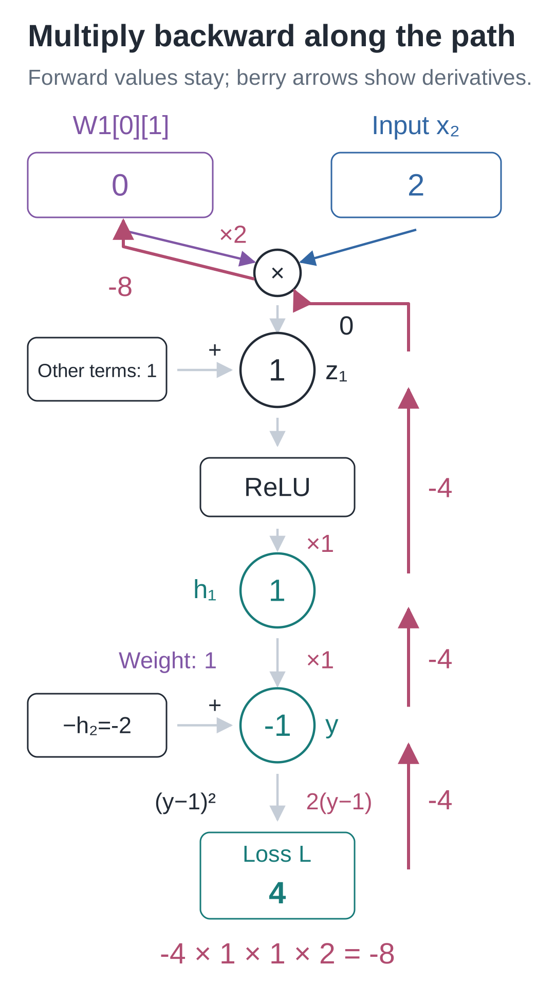
We are tracing just one weight path. The numbers on the berry-colored arrows are rates of change of loss with respect to the quantities along the path. The forward values 1 and 2 have not been overwritten, and the weight is still 0.
What about addition? If s=u+v, increasing only u slightly increases s by the same amount. The local derivative of s with respect to u is therefore 1, and its derivative with respect to v is also 1. The gradient arriving at s is multiplied by 1 and passed to each input; it is not divided between them.
If the same value branches out and affects the loss along two paths, a small increase changes both paths at once, so their effects must be added. This distinction is easy to reverse: an addition node passes its incoming gradient to each input; when one input receives gradients from multiple paths, those contributions are added. Multiply along one path; add when paths return to the same value.
For ReLU, the forward position determines the local derivative: it is 1 when z>0 and 0 when z<0. At z=0, there is no unique derivative. Our implementation chooses 0, matching the PyTorch convention used later.
How does the same −4 reach the other parameters?
Start at the output layer, where d_output=−4.
The inputs to its two weights are h₁=1 and h₂=2, so their gradients are −4×1=−4 and −4×2=−8. The output bias is added directly, so its gradient is −4.
To pass back to the two hidden values, multiply by their respective output weights:
∂L/∂h₁=−4×1=−4
∂L/∂h₂=−4×(−1)=4
Both z values are above 0, so ReLU's local derivative is 1, giving ∂L/∂z=[−4, 4]. Multiply each component by input [1, 2] to obtain the corresponding row of first-layer weight gradients.
| Parameter group | Original values | Corresponding gradients |
|---|---|---|
| W2 | [[1, −1]] |
[[-4, −8]] |
| b2 | [0] |
[-4] |
| W1 | [[1, 0], [0, 1]] |
[[-4, −8], [4, 8]] |
| b1 | [0, 0] |
[-4, 4] |
The gradient matrix has the same shape as the parameter matrix, so each gradient maps back to its corresponding parameter. In this example, each weight is used on only one multiplication edge. If a parameter is reused in multiple places, add the contributions it receives from all paths. We will use this in batch training.
The 18 extra forward passes needed for individual trial changes have now been replaced by one reverse-order calculation. The inputs and activation values it needs are still in the cache.
One update turns −1 into −0.2896
Once all 9 parameter gradients are ready, choose learning rate 0.01 and update them together using parameter−0.01×gradient:
W1 = [[ 1.04, 0.08],     b1 = [0.04, -0.04]
      [-0.04, 0.92]]
W2 = [[1.04, -0.92]]     b2 = [0.04]
A new forward pass gives hidden values [1.24, 1.76]:
prediction = 1.24×1.04 + 1.76×(−0.92) + 0.04 = −0.2896
L = (−0.2896−1)² = 1.66306816

The upper half of the diagram shows all gradients; the lower half shows the parameters after the joint update. The prediction has not yet reached target 1, but the loss has fallen from 4 to about 1.66. This new result must be recalculated using all the new parameters; the old hidden values cannot be reused.
Why not update each parameter as soon as its gradient is available? Later gradient calculations still read weights associated with the old forward pass. Updating midway would mix gradients from different parameter states within one round.
Watch the animated walkthrough
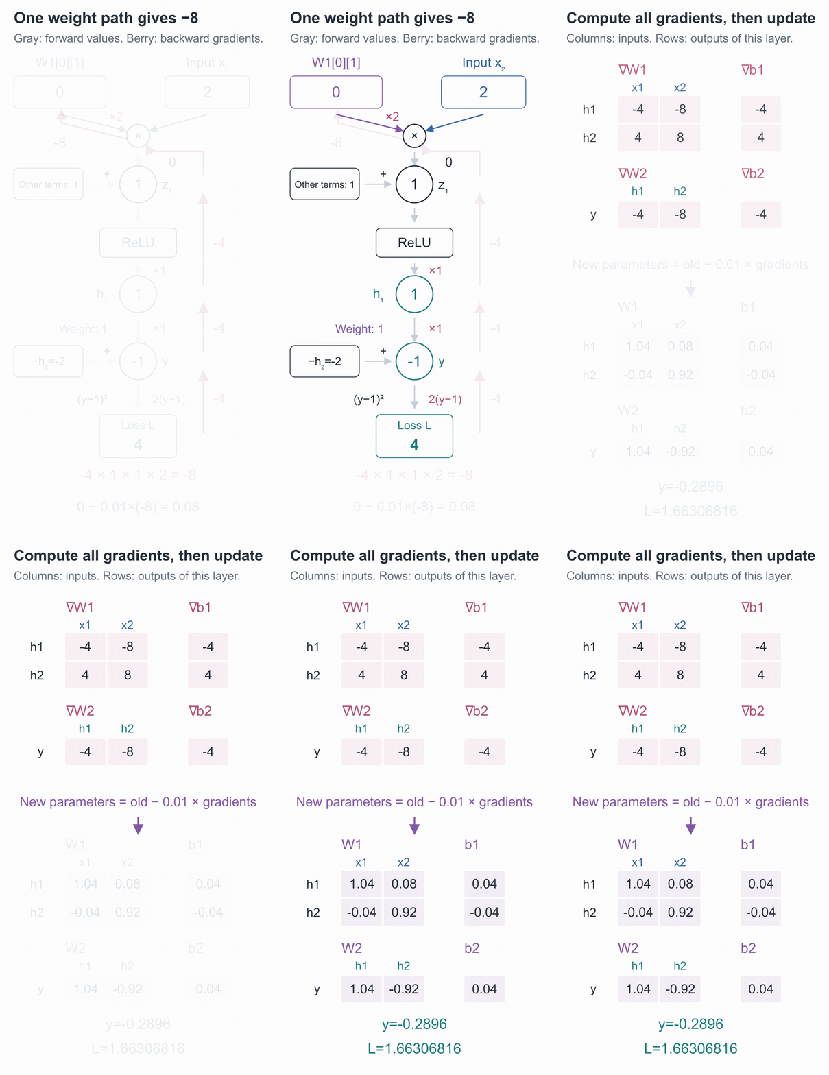
The animation follows the backward path through W1[0][1]. Parameters keep their old values until the update stage. Pause the interactive demo before the update to check: forward values are unchanged; only gradients have been added.
Try it here · Step-by-step experimentStep through the calculation, forwards or backwards.
Put the reverse-order calculation in a function
Run this from the companion code directory. forward reuses Lesson 03's implementation and returns a prediction and cache. hand_example returns this lesson's initial parameters, and step updates each parameter using the rule above. The new backward calculation is shown in full below.
from tiny_lm.manual_mlp import forward, hand_example, step


def backward(cache, target, params):
    """读取旧前向的缓存与参数,返回同形状的参数梯度,不更新参数。"""
    # 先求平方损失对最终预测的导数,供前面的各条路径共用。
    d_output = 2 * (cache["prediction"] - target)
    # 传回隐藏值时,分别乘上连接它们的输出权重。
    d_hidden = [d_output * weight for weight in params["W2"][0]]
    # ReLU 的局部导数:正区间传回原梯度,负区间与本实现的零点传回 0。
    d_z = [g if z > 0 else 0.0
           for g, z in zip(d_hidden, cache["z"])]
    return {
        # 权重梯度 = 该单元收到的梯度 × 这条权重所乘的输入。
        "W2": [[d_output * value for value in cache["h"]]],
        # 偏置直接相加,局部导数为 1,因此保留该单元收到的梯度。
        "b2": [d_output],
        "W1": [[g * value for value in cache["x"]] for g in d_z],
        "b1": d_z,
    }


# 固定一条训练题;hand_example 提供正文列出的那组初始参数。
x, target = [1.0, 2.0], 1.0
params = hand_example()
prediction, cache = forward(x, params)
gradients = backward(cache, target, params)
print("预测与损失:", prediction, (prediction - target) ** 2)
print("梯度:", gradients)
The d_ prefix is a naming convention; here it means the derivative of loss with respect to that quantity. d_hidden multiplies the output gradient by the corresponding weight. d_z uses the forward value z to decide whether the gradient passes through ReLU. Finally, each layer's weight gradients are “the gradient received by this layer × this layer's input.”
backward stores the gradients calculated by these local rules in a new dictionary and does not modify params. step still handles parameter updates.
Change it. Run it. See what happens.
Start with the chapter’s parameters. Update once, then try ten steps.
Edit Python code
Tab indents; Shift + Tab unindents. Press Esc then Tab to leave the editor. Ctrl / ⌘ + Enter runs the code.
Run the code to see the result below.
Ready to run…
Perturb that weight to check −8
Finite differences are slow, but they provide an independent check of the backward code. First, check only the path we traced, W1[0][1], while keeping the other parameters fixed:
# 接着上一段,x、target、params、gradients 仍对应同一次旧前向。
epsilon = 1e-5
old_value = params["W1"][0][1]
# 只试改第一行第二列的权重,其余参数保持原值。
params["W1"][0][1] = old_value + epsilon
plus = (forward(x, params)[0] - target) ** 2
params["W1"][0][1] = old_value - epsilon
minus = (forward(x, params)[0] - target) ** 2
# 先恢复原值,再把差分导数与反向得到的同一项梯度比较。
params["W1"][0][1] = old_value
numerical = (plus - minus) / (2 * epsilon)
print("差分与反向:", numerical, gradients["W1"][0][1])
assert abs(numerical - gradients["W1"][0][1]) < 1e-7

# 全部梯度都来自旧参数;统一更新后,重新前向,不能沿用旧隐藏值。
step(params, gradients, learning_rate=0.01)
new_prediction, _ = forward(x, params)
print("更新后:", new_prediction, (new_prediction - target) ** 2)
# 约为 -0.2896、1.66306816
Increase the value slightly, decrease it slightly, and restore it after the calculations. Only then run step. Both gradient results are close to −8. The companion program keeps a complete check of all 9 parameters using the same principle.
Finite differences check the calculation at the current point. Both z values here are far enough from 0 that tiny perturbations do not cross ReLU's bend. At the bend itself, a central difference need not equal the derivative chosen by the program, so the same error threshold is not a suitable correctness test there.
Two tracing exercises
- Increase only
W1[0][1]by 0.001, leaving all other parameters at their initial values. What are the new prediction and loss? Estimate the loss change using gradient −8. How far is the estimate from the actual change? - Keep the original parameters, but change the output to
y=h₁−h₂+h₁, with target still 1. What is the gradient of loss with respect toh₁? What would be missed by following only oneh₁path?
Reference answers
Answers: For the first exercise, the new prediction is −0.998, and the loss is 3.992004. The gradient estimates a change of −8×0.001=−0.008; the actual change is −0.007996, a difference of 0.000004. For the second, the current y=0, so ∂L/∂y=−2. Each of the two addition paths from h₁ contributes −2, making the total gradient −4. Following only one path misses the other −2; effects from the same value must be added.

There is only one h₁ at the top of the diagram, branching into two uses below. During backpropagation, both −2 contributions return to it. They must not be averaged to −2, and the later contribution must not overwrite the earlier one.
In the next lesson, we will switch to PyTorch, first check these hand calculations, and then observe the network's predictions after 500 updates.
Run this from the code directory:
# 在配套代码目录运行本讲实验,核对正文中的结果。
python -m lessons.l05
Companion resources: Entry point · Handwritten implementation · Interactive demo
Source navigation: manual_mlp.py · backward.