Two parameters, one loss

Prediction = 2w + b · L = (2w + b − 6)²

3D surface of weight w, bias b and squared loss L

3D is unavailable. This image is a static reference; numerical controls still work.

Loss surfaceSlice b = 0Sampled loss pathCurrent pointGround −gradient direction

Prediction2

Loss16

Updates0

Weight w

Bias b

Learning rate η

Start at w=1, b=0. Choose a learning rate, then compare the two updates.

Calculation, update log and notes

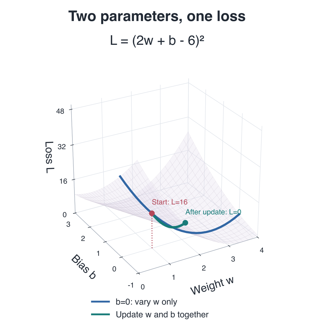
The input stays at 2 and the target at 6. The ground axes are parameters w and b; height is the same squared loss. The valley satisfies 2w+b=6, so one problem cannot uniquely determine both parameters.

Only the endpoints perform a parameter update. The green path samples 64 intervals along the straight parameter segment between old and new values, recalculating L at every sample. It shows loss while crossing the valley; it is not a straight line between endpoint losses. The yellow arrow shows the direction of −∇L in the parameter plane, with its length scaled for display.

From w=1, b=0, rate 0.1 gives L=0.64 for w only, or L=0 for both. Rate 0.3 gives L=31.36 for w only, or L=64 for both. An oversized step crosses the valley. Both derivatives are calculated at the same old point.

The initial view is fixed, so a finger can scroll the page over the plot. Enable rotation to drag. With the plot focused, arrow keys rotate and Home resets the view. All data, calculations and graphics work offline.

Plot domain (linear height scale)

Updates

Step	Changed	Parameters (w, b)	Loss L

No update yet.

Data and formula: code/artifacts/lessons/l04.json · Open the original static figure ↗

Enable JavaScript to edit parameters, or inspect the static figure first. Open the original static figure.view-tools{display:none}